
1. Introduction
There are different approaches available for modal analysis of general concrete gravity dam-reservoir systems in the frequency domain. Some are dependent on sub-structuring techniques and employ the mode shapes of the dam with an empty reservoir [1], while a more direct approach relies on the mode shapes of the coupled dam-reservoir system. However, in this latter alternative, standard eigenvalue computation methods are not applicable due to the fact that the coupled system is not symmetric [2]. Although it is possible to achieve the symmetrisation, it requires introduction of additional variables and complications in computer programming [3, 4].
In the present study, a modal analysis method is proposed which is dependent on mode shapes evaluated from the symmetric part of the original eigen-problem of the system. The formulation of this method is presented initially and a special computer program “MAP-76” [5], is enhanced based on this approach. The program was originally developed based on direct method in frequency domain and in this way the modal analysis option is also included. Utilising this tool, the frequency response functions are calculated for an idealised triangular dam as an example. The convergence of the method is controlled for normal compressible water with different assumptions imposed at the reservoir bottom, as well as for a pseudo-incompressible impounded water condition.
2. Method of analysis
The modal analysis technique utilised in this study is designed for the FE-(FE-HE) concept of discretisation (i.e., Finite Element – (Finite Element-Hyperelement)), which is applicable for a general concrete gravity dam-reservoir system. In this manner, the dam is discretised by plane solid finite elements. While, the reservoir is divided into two parts, a near field region (usually an irregular shape) in the vicinity of the dam and a far field part (assuming constant depth), which extends to infinity. The former region is discretised by plane fluid finite elements and the latter part is modelled by a two-dimensional fluid hyperelement.
The formulation could be explained much easier, if one concentrates initially on a dam with finite reservoir system (basically the same as a model of dam and reservoir near field), and subsequently add the effects of reservoir far field region for the more complicated case. For this purpose, let us begin with this simpler formulation and then complete it on that basis.
2.1 Dam with Finite Reservoir System
This is the problem, which can be totally modelled by finite element method. It can be easily shown that in this case, the coupled equations of the system may be written as [6]:

(1)
M, C, K in this relation represent the mass, damping and stiffness matrices of the dam body, while G, L, H are assembled matrices of fluid domain. The unknown vector is composed of r, which is the vector of nodal relative displacements and the vector p that includes nodal pressures. Meanwhile, J is a matrix with each two rows equal to a 2 2 identity matrix (its columns correspond to unit rigid body motion in horizontal and vertical directions) and ag denotes the vector of ground accelerations. Furthermore, B in the above relation is often referred to as interaction matrix.
The relation (1) can also be written alternatively in a more compact form as:

(2)
where

are defined as follows:

(3)

(4)
Meanwhile, the exact form of

are well apparent by matching relations (1) and (2) together. Obviously, these matrices can also be written as sum of the symmetric and unsymmetric parts as below:

(5a)

(5b)

(5c)
It is noted from equation (1) that the damping matrix is totally symmetric, and the following relation also holds:

(6)
For harmonic ground excitations

displacements and pressures will all behave harmonic, and the equation (2) can be expressed as:

(7)
In direct frequency domain method, this relation is solved for unknown vector

at different frequencies. Although, the total dynamic stiffness matrix (resulting left hand side matrix of relation (7)) is not symmetric, it can be easily made symmetric [6]. Therefore, usual symmetric skyline solvers can be employed utilising complex number arithmetic.
In modal approach, which is the basis of the present study, the method relies on obtaining the natural frequencies and mode shapes of the system. Thereafter, the solution can be estimated as usual based on the combination of these modes.
Decoupled Modal Technique
The eigenvalue problem corresponding to relation (2) can be written as follows:

(8)
Physically, it is clear that the eigenvalues of this system are real and free vibration modes exist. However, it is noted from the form of matrices

(relation (5)) that the system is not symmetric and standard eigenvalue computation methods are not directly applicable. Although there are techniques available to arrive at a symmetric form and reduce the problem to a standard eigenvalue one, it is computationaly costly and additional variables are required to be introduced. Therefore, this path is not pursued in the present study. As a substitute, it was preferred to work with the eigenvalues and vectors extracted from the following eigen-problem:

(9)
Where Ks, Ms are the symmetric parts of the

matrices, as mentioned previously (relation (5)). Of course, the eigenvectors obtained through the above relation are not the true mode shapes of the coupled system. However, these can be presumed as Ritz’ vectors which can be similarly combined to estimate the true solution. The solution of this substitute eigen-problem are easily obtained by standard methods, since the involving matrices are symmetric and positive definite. Having the orthogonality condition and normalising the modal matrix with respect to mass matrix, one would have:

(10a)

(10b)
Where I is the identity matrix and

is a diagonal matrix containing the eigenvalues of the symmetric substitute system. The following relations are also derived easily based on relations (5), (6) and (10):

(11a)

(11b)
As usual in modal techniques, the solution is written as a combination of different modes:

(12)
The vector Y contains the participation factors of the modes. Substituting this relation into (7) and multiplying both sides of that equation by XT, it yields:

(13)
Or alternatively, the following relation is obtained by employing (11):

(14)
In this relation, additional matrix definitions are utilised as below:

(15a)

(15b)
The vector of participation factors can be solved through relation (14), which is dependent on the excitation frequency. Thereafter, the unknown vector is obtained by equation (12) as usual in modal procedure. It must be mentioned that the left hand side matrix of relation (14) is in general unsymmetric. However, it may be easily transformed to a symmetric matrix by multiplying certain rows of that matrix relation by an appropriate factor. This can be shown as follows:
It is noticed through (1) and (5) that the symmetric matrices utilised in the substitute eigen-problem, corresponds to the decoupled dam-reservoir system. Therefore, the natural frequencies and eigenvectors are actually related to this decoupled system. It should be noted that in actual programming, one can modify the usual subspace iteration routines to converge to the desired lowest modes of the dam first, and similarly for the finite reservoir region afterwards by appropriate selection of initial vectors. Meanwhile, they can also be obtained as two separate problems. Let us now assume for simplicity, without loss of generality that the mode shapes for the dam are ordered first and the ones for the finite reservoir considered subsequently in the modal matrix,

(16)
and similar arrangements for the eigenvalues in the diagonal matrix.

(17)
Then, it is clear that the following relations hold:

(18a)

(18b)

(18c)
Of course, it must be mentioned that in the last relation, it is assumed that the damping matrix of the dam is of hysteretic type. This means:

(19)
Where

is the constant hysteretic factor of the dam body.
Substituting relations (18) into (14), the following equation is concluded:

(20)
It is noticed that, the vector of participation factors is also assumed to be partitioned into two parts in this relation, and as before the indices 1, 2 correspond to dam and reservoir modes, respectively. Relation (20) is equivalent to (14) and as mentioned previously, this is in general an unsymmetric system of equations. However, it is now revealing that this matrix relation could become symmetric by multiplying the lower matrix equation by a factor of , which yields the following relation:

(21)
2.2 Reservoir Hyperelement
In previous studies [6, 7], the hyperelement was assumed to be formulated in terms of relative horizontal displacement degrees of freedom located at the vertical reference plane of the element. For direct method of analysis in frequency domain, a second approach could also be adopted in which the horizontal displacements are replaced by nodal pressure degrees of freedom. In direct approach, both of these alternatives are acceptable and have their own advantages. However, in modal analysis, one is almost forced to use the second approach, since the first approach encounters difficulty due to the fact that all modes have zero components corresponding to these horizontal displacement degrees of freedom. Of course, one can still use the first approach, if the fluid hyperelement horizontal displacements are also considered as unknowns in addition to the modal participation factors. However, this makes the procedure relatively inefficient. Therefore, in the following, the formulation for this second approach is discussed. It should be also mentioned that all the basic relations utilised in this section, are extracted from the previous work [7], since they are common in both formulations.
As it was shown in the previous study [7], the eigenvalue problem related to the hyperelement must be solved as the first step. Meanwhile, there exists a particular solution,

which corresponds to uniform unit vertical acceleration of reservoir bottom. In that case, the solution is independent of x-direction, and this solution can be obtained by setting the wave number (k) equal to zero in corresponding relations [7]. Thereafter, the vector of pressure amplitudes for the hyperelement reference plane can be written as,

(22)
with the help of following definitions for reservoir modal matrix and vector of hyperelement participation factors:

(23a)

(23b)
While, the modal matrix satisfies the orthogonality condition and it is also normalized with respect to matrix A , appearing in hyperelement eigen-problem.

(24)
Moreover, the fluid hyperelement horizontal accelerations vector for the reference plane is given as [7]:

(25)
Solving for participation vector from (22) by employing orthogonality relation (24) of modal matrix and substituting in (25) yields:

(26)
Multiplying both sides of this relation by , one obtains:

(27)
With the help of following definitions:

(28a)

(28b)

(28c)
represents a consistent vector equivalent to integration of inward horizontal acceleration for the hyperelement and this vector contains essentially similar quantities as the components of the right hand side vectors of usual fluid finite elements. Of course, the relation (27) can also be written as below,

(29)
by employing the following matrix definitions:

(30a)

(30b)
2.3 Dam-Reservoir System
The formulation for a dam with finite reservoir, was already presented. For the case where the reservoir extends to infinity, a hyperelement must be used along with the fluid finite elements utilised for reservoir near field. Meanwhile, the governing relation for hyperelement was derived in previous section. Therefore, if the matrices of the hyperelement assemble in conjunction with the fluid finite elements, equation (7) would now become:

(31)
Where

are the expanded form of

matrices which cover the entire fluid domain pressure degrees of freedom. Assuming that the pressure degrees of freedom related to hyperelement are ordered first in the unknown pressure vector, then these matrices would have the following forms:

(32a)

(32b)
The relation (31) is the equation to be used instead of (7), when the reservoir is extended to infinity and one is considering the direct approach in frequency domain. Then, it is easy to see that in modal analysis, the relation (21) must be modified as follows when the hyperelement is also included.

(33)
3. Modelling and Basic Parameters
A special computer program “MAP-76” [5] is used as the basis of this study. The program was already capable of analysing a general dam-reservoir system by direct approach in the frequency domain [6]. In this study, the modal analysis option is also included in the program based on the formulation presented in the previous section.
The program is based on the FE-(FE-HE) concept. Meanwhile, there are two alternatives available for the hyperelement in the direct approach. That is using the horizontal fluid displacements or the pressure degrees of freedom. However, in modal approach, only the second alternative is implemented, since the other option is not efficiently applicable.
3.1 Model
An idealised triangular dam with vertical upstream face and a downstream slope of 1:0.8 is considered under a full reservoir condition, and assuming a rigid foundation. The discretisation of the dam-reservoir system is displayed in Fig. 1.
The dam is discretised by 20 isoparametric 8-node finite elements, which are assumed in a state of plane strain. The reservoir is divided into two parts. A length of the reservoir equal to water depth is considered as the reservoir near field region, which is modelled by 100 isoparametric 4-node fluid finite elements. The reservoir far field is treated by a fluid hyperelement having 11 nodes with pressure degrees of freedom.
3.2 Basic Parameters
The dam body is assumed to be homogeneous and isotropic with linearly viscoelastic properties for mass concrete: Elastic modulus (Ed ) = 27.5 GPa., Poisson’s ratio = 0.2, unit weight = 24.8 kN/m3, and

hysteretic damping factor = 0.05.
The impounded water is taken as inviscid fluid with unit weight = 9.81 kN/m3. The water is initially assumed as a compressible fluid with a pressure wave velocity c=1440.m/sec. However, in a later stage, the incompressible case is also treated. For this purpose, a relatively high value of c=1440.x106m/sec, is considered as a substitute for the actual infinite value. This is referred to as the pseudo-incompressible case.
4. Results
As mentioned, the water is initially taken as a compressible fluid with its normal pressure wave velocity of c=1440.m/sec. As a first step, the eigen-problem is solved based on the symmetric parts of the total mass and stiffness matrices. This is actually a decoupled system, and the natural frequencies obtained correspond to either the dam or the finite reservoir (reservoir near field) region. Similar to the values for the dam withan empty reservoir, or the natural frequencies of the finite reservoir assuming rigid boundaries except at the water surface. The first five natural frequencies of each domain are listed in Table 1.
It is noticed that the first natural frequency of the finite reservoir is actually lower than the one corresponding to the dam. Meanwhile, the natural frequencies of the dam are wider spread in comparison to the ones related to the finite reservoir domain. This means that a much higher number of modes are required for the finite reservoir in comparison with the dam, in order to obtain an accurate solution for the practical range of frequencies of interest.
The first mode shape of the dam is displayed in Fig. 2. Meanwhile, the first two mode shapes of the finite reservoir region are depicted in Fig. 3. It is noticed that the first mode of the finite fluid domain corresponds to a case where pressures are constant in the horizontal direction. In other words, this mode is symmetric and independent of the horizontal direction. Meanwhile, the second mode is exactly anti-symmetric.
In the next step, the modal analyses are carried out based on two different set of modes employed. The first case corresponds to a set of 10, 25 modes utilised for the dam and the reservoir near field domains, respectively. In the second case, these numbers are increased to 20, 50 modes. Of course, at this step the hyperelement is also considered to model the effects of reservoir far field.
As mentioned, the foundation is assumed rigid in the present study. However, two different alternatives of reservoir bottom absorption coefficient

and 0.5 were also investigated.

represents full reflection, while

allows for partial refraction waves impinging at reservoir’s bottom [7, 8].
The response of horizontal acceleration at dam crest due to horizontal and vertical harmonic ground excitations are obtained for different cases, and the results are presented in Figs. 4 and 5 for

values of 1 and 0.5, respectively. In each graph, the response obtained by the corresponding direct approach is also shown for comparison purposes. Meanwhile, it should be mentioned that the horizontal axes in these graphs are normalised with respect to

(the first natural frequency of the dam with an empty reservoir).
When

(Fig. 4), It is noticed that the modal solution is converging to the exact solution (direct approach results) as the number of modes increase. Meanwhile, it is clear that the errors are negligible for the frequency range considered (up to approximately five times

even for the set of 10, 25 modes employed. This means that from practical point of view, one can obtain accurate solutions with a relatively low number of mode shapes in each domain. Similar observations are noted for the

cases (Fig. 5).
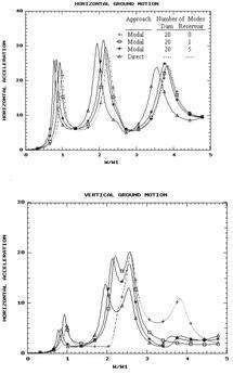
Following from this, the pressure wave velocity is increased to a relatively high value of c=1440.x106m/sec. As mentioned, this can be envisaged as a pseudo-incompressible case. Again, the responses are compared for different sets of number of modes, against the response obtained based on the direct approach (Fig. 6). The convergence trend is quite evident similar to previous cases. Meanwhile, it is proved that the technique can be employed to obtain the incompressible solution by modal approach without any difficulty or special requirements. Finally, it seemed interesting to study the results that could be obtained for this pseudo-incompressible problem if one employs very low number of finite reservoir modes. For this purpose, the number of modes utilised for the dam is fixed (20 modes) and three cases are considered corresponding to 0, 1 and 5 modes for the finite reservoir region.
The results are compared in Fig. 7 along with the direct approach solution. Of course, it is clear that the response obtained with no mode of the finite reservoir region being considered, is actually the same as the response of the dam with an empty reservoir. It is noted that the first peak is occurring at

(the first natural frequency of the dam with an empty reservoir) in this case as expected.
Again, it is noticed that the responses are shifting toward the true solution (direct approach results) as the number of combined modes increase. However, even with five modes, the accuracy is not acceptable. This is in spite of the fact that the first natural frequency of the finite reservoir region for this pseudo-incompressible case is several orders of magnitude higher than the first natural frequency of the dam. Therefore, it is noted that the number of modes required for the reservoir near field region does not necessarily decrease for the pseudo-incompressible case. Although accurate solutions can be obtained with relatively low number of modes for the reservoir near field region (Fig. 6), the accuracy is not acceptable if very low number of modes of that region is employed (Fig. 7).
5. Conclusions
A formulation is presented for the dynamic analysis of general concrete gravity dam-reservoir systems in the frequency domain. The method is based on the modal approach applied for the FE-(FE-HE) technique (i.e., Finite Element-(Finite Element-Hyperelement)). The special computer program MAP-76 is modified based on the theory explained and the dynamic behavior of an idealized triangular dam with vertical upstream face is considered as a controlling example. The water is initially assumed compressible with a normal pressure wave velocity of m/sec. Subsequently; this is increased to a relatively high value ( m/sec.), which is referred to as the pseudo-incompressible case. Specifically, this investigation leads to the following conclusions:
• For the normal compressibility condition, it is controlled that the modal solution converges to the exact solution (direct approach results) as the number of modes increase. It is observed that the errors are negligible for the frequency range considered (up to approximately five times the natural frequency of the dam with an empty reservoir), even for the low set of 10, 25 modes selected for the dam and the reservoir near field region, respectively.
• For the pseudo-incompressible case, it is noted that the number of the modes required for the reservoir near field region does not decrease in comparison to the normal compressible water case. Meanwhile, the accuracy is not acceptable if very low number of modes is utilised for this fluid region. This is in spite of the fact that the first natural frequency of the finite fluid region for this pseudo-incompressible case is several orders of magnitude higher than the first natural frequency of the dam. However, accurate solutions can still be obtained with relatively low set of number of the modes similar to the normal compressible case.
• The formulation introduced is proved to be an effective and convenient procedure for dynamic analysis of general concrete gravity dam-reservoir systems based on the modal approach in frequency domain. The method is not dependent on non-standard eigenvalue extraction routines, while it converges to the exact solution if all the modes are considered. Furthermore, it is also shown that the technique can be employed to obtain the solution for the incompressible case without any difficulty or special requirements.
Author Info:
Vahid Lotfi, Associate Professor of Civil Engineering Department, Amirkabir University, Tehran, Iran
TablesTable 1


