P Krishnamachar and Arpad Fay investigate the effect of surface roughness on losses and performance of hydraulic turbines
Equation 1
Hydraulic energy conversion into mechanical energy in a hydroturbine is inevitably associated with energy losses. Energy losses depend upon the type of turbine, its design, size (dimensions) of the turbine and regime of operation. Hydraulic turbines are very efficient prime movers. Modern powerful reaction turbines have high values of overall efficiency of 92% to 96% at design-point operation and 86% to 91% at rated regimes. Nevertheless, further improvement of efficiency, especially at off-peak regimes of overload and part-load operation is important and constantly sought, because even 0.1% increase in efficiency of powerful modern machines gives a substantial increase in annual output of electrical energy. For a medium head Francis turbine of 185,500kW output capacity working at a power factor of 0.6, 0.1% higher efficiency may be worth US$117,000 of additional annual revenue at US$0.12/kWh, the capitalised value of which may be about US$1.5M per unit. Also, it was estimated that 1% difference in efficiency of a Kaplan turbine was equivalent to 10% of turbine price.
To improve the performance of such efficient turbines, it is necessary to investigate all the hydraulic elements and runner in particular, to study the nature of losses and to find means of reducing them. Fluid friction losses – especially in the runner where the relative velocities are the greatest – need special consideration. The flow conditions in a hydraulic turbine, especially the prototype turbine, are such that the friction factor is a function of the relative roughness only. Therefore the roughness protrusions of the runner surfaces in contact with the flow are very important and should be the least. Greatest care is hence taken in casting and finishing these surfaces and these operations consume a great deal of time and costs..
Losses in hydraulic turbines and scaling up from model to prototype
In scaling up hydraulic efficiency of turbine hh from model to prototype, it is generally accepted as a standard practice that the hydraulic losses can be divided into two parts: the part due to kinetic losses arising from vortices etc., that needs no scaling up and the other due to fluid friction which is to be scaled up. Hydraulically smooth flow can be achieved in the model turbines at the velocities generally prevailing by limiting boundary surface roughness ( RMS – root mean squire – value of roughness protrusions ) Ra typically to 0.4 microns in runner and guide wheel achievable through suitable surface finish. Limiting roughness for hydraulically smooth flow through other components is about 2.5 times this value.
For scaling up model efficiency to homologous prototype turbine assuming hydraulically smooth flow, several expressions obtained by various investigators based on their experiences are available. Those expressions based on the concept of subdivision of internal losses into the scaled up and non-scaled up parts take the general form given by Ackeret, Hutton and Osterwalder.

(1)
where: ?h is hydraulic efficiency, ?h relative hydraulic loss = 1-?h , Re is Reynolds number, V is loss distribution coefficient, M and P refer to model and prototype turbines.
The index a and loss distribution coefficient V are based on experience. The international-electrotechnical-commission (iec), International Association for Hydraulic Research (iahr) and their working groups collected and analysed vast data on both model and prototype turbines. Hutton gave values of 0.7 for V and 0.2 for a applicable to Kaplan turbines. Osterwalder gave a=0.16 applicable to all reaction turbines and rotodynamic pumps. IEC [1] specified V=0.7 for Francis turbines and pump-turbines operating in turbine mode. Based on a critical study of both experimental and analytical data, Fay [2] gave an average equation:

(2)
nq is the specific speed based on speed n in rpm, discharge Q in m3/sec and head H in meters. Any characteristic velocity like u2 the peripheral velocity at the runner diameter at exit can be taken to calculate Re as only the ratio of Re is involved and velocity ratio is constant in homologous turbines. Equation [1] gives the efficiency of hydraulically smooth prototype turbines. However, most prototype turbines operate in hydraulically rough regime of flow.
Computation of effect of boundary surface roughness in prototype turbines
In computing the effects of roughness of surfaces in flow passages on the efficiency of prototype hydraulic turbines, a two-step method suggested by Osterwalder can be adopted. In the first step, from the hydraulic efficiency of a tested homologous model, the hydraulic efficiency of the prototype turbine is calculated for hydraulically smooth flow using appropriate step up formulau (Equations 1&2). In the second step, from the hydraulic efficiency ?h smooth of the prototype turbine calculated for operation in hydraulically smooth flow regime, the hydraulic efficiency ?h rough for operation of the prototype turbine in hydraulically rough regime at the same Reynolds number is calculated. The total relative hydraulic loss ?h in the turbine space is the sum of the relative losses in individual elements i.e. the relative losses in the spiral casing (?sp), stay ring (?st), distributor (?d), runner (?r) and draft tube (?d.t).

(3)
Where, ? H is the part of turbine head lost in overcoming the hydraulic resistance. Combining the vanes treated as plates together and considering disc friction losses,

(4)
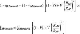
The equation for calculation of ?h rough from ?h smooth resulting from an analysis by Hutton and Fay can be used after suitable modifications considering different loss distribution coefficients for different components.

(5)
where sp denotes spiral casing, v the vanes, r the runner, dt the draft tube d the disc and ? the friction factor.
Values of the component distribution coefficient V have been estimated from the extensive experimental and analytical data for Francis turbines from JSME [3] and Osterwalder [4].
Friction factor for hydraulically smooth and rough boundaries, ?smooth and ?rough for each component at the same Reynolds number are derivable from the relevant expressions or charts. Substituting the values V and ? thus obtained into equation (5), 1-?hPrough = ?hPrough can be derived.
To study the effect of surface roughness on the hydraulic losses or efficiency, it is not necessary to calculate values of ?. It can be seen from equation (5), that it is only necessary to calculate the ratios of ?rough to ?smooth. Examining the Colebrook and White formula for pipe friction valid for random commercial roughness:

(6)
where ks is equivalent sand roughness and D the diameter,
or its modification by Fay [2,5]

(7)
A varying from 0.65 to 0.9 depending on the type of roughness, and the flat plate friction formulau

(8)
where cf is drag coefficient and L the length of the plate, a universal roughness law is evolved by Fay[2,5]:

(9)
where Raactual is the root mean squire (RMS) value of roughness protrusions of the prototype component for which ?rough / ?smooth is to be calculated for substitution in equation (9) and Rachar is a characteristic roughness equal to C2 ?/w with C2 as a constant, ? as kinetic viscosity and w as the characteristic velocity, the same as for Re. Ra = ks / 1.7 established by Nixon and Cairney [6]. The values of coefficients and index are shown in table 2 for various components of turbine:
These modified equations by Fay give better fit for ground surfaces. Limiting conditions for hydraulically smooth flows can be obtained when ?rough / ?smooth =1. Substitution of this condition in to Equation [9] yields Raactual / Rachar =1-A = 0.25. Therefore:
If Raactual / Rachar = 1-A = 0.25, the flow is hydraulically smooth, and lrough = lsmooth
If Raactual / Rachar > 1-A = 0.25, the flow is affected by roughness and, ?rough / ?smooth can be obtained for various values of Raactual by solving Equation [9]. By substituting ?rough / ?smooth and values of V into equation [5], 1-?hPrough or relative losses ?hPrough in a rough prototype turbine can be evaluated.
Example of effect of roughness on prototype efficiency
The example chosen is Vevey’s Francis turbine at Serre-Poncon, France. Published / derived details from Lucien Vivier [7] and Th. Bovet [8] are:
• Head H = 124.5m, Discharge Q = 75m3/sec, Speed n = 214 rpm, Power P = 83,900kW
• Efficiency h = 91.6%, Specific speed with P in hp ns = 177 rpm, nq = n Q1/2 /H3/4 = 49.72.
• Inlet to spiral casing = 3.7m diameter, Characteristic velocity w = 75/(p3.72/4) = 6.975m/sec
• Guide vane pcd D0 = 4.17m diameter, Height b0 = 0.679m, GV angle with radius = 450
• Characteristic velocity for guide vanes w = 75/(4.17p0.679)sec 45º= 11.867m/sec.
• Runner exit diameter D2 = 3.197m, Characteristic velocity for runner w = p3.197(214/60)=35.822m/sec.
• Draft tube inlet diameter D2 = 3.197m, Characteristic velocity w = 75/(p3.1972/4) = 9.372m/sec.
• Max. runner diameter at seals = 3.58m, Characteristic velocity for disc w=p3.58(214/60)=40.11m/sec.
Kinetic viscosity n used in computations =10-6 m2/sec.
The spiral casing and draft tube are made of welded steel plates and are coated with bituminous or epoxy paint. Their equivalent sand roughness ks is 1.5 micron and Ra is 0.9micron. They are assumed to be maintained as such. The guide vanes and runner are ground and polished. Effect of different degrees of grinding and corresponding roughness is shown in these computations.
The parameters for computations are shown in table 3, A being 0.75 for all components of prototype:
Letting ?rough / ?smooth = X , relevant values are substituted in equation [9] for each component and X solved for by successive approximations.
• Spiral casing, 0.10462683=X8-0.75/X0.5 is solved to get X=0.9815572, VX=0.08834048 *
• Guide vanes, 0.18987041 =X7-0.75/X0.5 is solved to getX=0.9916538, VX=0.10908192 *
• Runner, 0.57314822=X7-0.75/X0.5 is solved to get X=1.0392004, VX=0.21199688
• Draft tube, 0.14058 =X8-0.75/X0.5 is solved to get X=0.986333, VX=0.01183600 *
• Disc friction, 0.35653802=X5-0.75/X0.5 is solved to get X=1.0191448, VX=0.07134014
S VX =0.49259484
Substituting in equation (5),

(10)
or

(11)
?P = 91.6% or ?P = 8.4%. Considering mechanical losses to be 0.9%, ?hP = 7.5%.
If this is taken as without roughness considered,

(12)
Increase in ?hP = drop in ?hP = 0.04946% .
For various values of surface roughness Ra for ground components, the computed drop in efficiency of rough prototype turbine are shown in table 4.
Accuracies, uncertainties and allowances
Accuracy in the determination of hydraulic efficiency of the prototype turbine from field tests ranges from 1% to 2%. Or the relative hydraulic losses 1-hhPrough or zhPrough are thrown into an error of 0.12% to 0.25%. Therefore determination of loss distribution coefficient V based on such prototype test data is also subject to high uncertainty. Further refinement of scaling up calculations are therefore not warranted at this stage. Various scaling up procedures recommended are for customers to assess bids or estimates of prototype performance from witness model tests and not for design developments. Designers in manufacturing firms are already adopting sophisticated computational methods for the analysis of boundary layer development and drag from computed velocities over the surfaces of various components. Better methods of scaling up can be expected in due time.
Model tests are considered very accurate with error in determination of model efficiency of ±0.2%. Models are made as smooth as possible to ensure hydraulically smooth flow. But the measured efficiency changes due to roughness are also small. The uncertainties in the estimates of prototype efficiency are:
• With constant V and without considering roughness effects: ±0.83%
• Considering variation of V with nq (eq.2) but without roughness effects: ±0.65%
• With constant V but considering roughness effects: ±0.69%
• Considering both variation in V and roughness effects: ±0.46%
The scaling-up procedures to obtain prototype efficiency are based on values of V which are good averages for turbines with the same nq and on the assumption that turbines are equally sensitive to roughness as pipes, discs and plates. The V values may differ for uncommon designs. The above estimates of uncertainties include such differences.
From computations exemplified corroborating with the results obtained earlier by Fay[2], it can be seen that, if a decimal point of efficiency is considered in deciding on bids, the roughness of ground surfaces will have to be limited to about 1 micron. Finishes to 3.2 microns as limited by IEC code 60193 of 1999 [9] may result in efficiency losses of the order of 0.4% (reference table 4). Loss of efficiency of 0.5% threshold recommended for repair of turbines affected by cavitation pitting amounts to about 5 microns of equivalent surface roughness.
Conclusions
The paper synthesizes analytical procedures with practical data and provides a reasonably simple computational method to obtain realistic estimates for roughness effects on the optimum efficiency of Francis turbines. The universal roughness law evolved to study the effect of surface roughness on the hydraulic losses or efficiency gives better fit for ground surfaces of a turbine. Making the reasonable assumption that turbine components are equally sensitive to roughness as pipes, plates and discs, the changes in prototype efficiencies due to roughness computed by the proposed method provide the minimum changes that can be expected. The method provides a more reliable tool for closer assessment of offers. The computational procedure can be used by manufacturers to set a degree of finish for the turbine to achieve the required degree of change in prototype efficiency due to roughness and by maintenance engineers to fix maintenance schedules. Model tests still remain more accurate than field tests.
Table 1 Table 2 Table 3 Table 4 (1) Equation 1 (2) Equation 2 (3) Equation 3 (4) Equation 4 (5) Equation 5 (6) Equation 6 (7) Equation 7 (8) Equation 8 (9) Equation 9 (10) Equation 10 (11) Equation 11 (12) Equation 12 Author Info:
P.Krishnamachar, Hydro Consultant, 1208 Hogan Drive, South Plainfield, New Jersey 07080, US and Arpad Fay, Chief Consultant (Retd), Ganz Mawag, 33 Szent Donat ut H-2097, Pilisborosjeno, Hungary. Email: pkrishnamachar@rediffmail.com and arpad.fay@axelero.hu